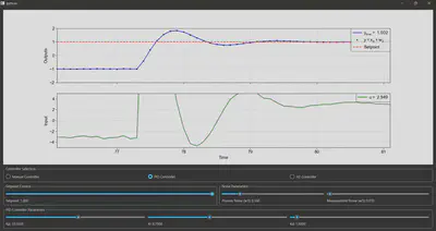
Interactive Control System
Write-up coming soon…! Code available on GitHub here in the meantime.
The plant
The plant I chose to implement in the program comes from Question 2 of the final exam for the 4th year (Part IIB) Optimal Controls (4F3) class of 2021 at University of Cambridge (availiable here), whose cribs I used to verify my controller implementations. This is a two-compartment model of drug diffusion in a person’s body, with the following variables:
- $ x_1 $: drug concentration in compartment 1 (state 1)
- $ x_2 $: drug concentration in compartment 2 (state 2)
- $ y $: measured drug concentration in compartment 2 (measured output)
- $ u $: drug injection into compartment 1 (control input)
- $ w_1 $: drug concentration disturbance in compartment 2 (process noise)
- $ w_2 $: measurement disturbance (measurement noise)
The process dynamics are described by the following ordinary differential equations (ODEs):
$$ \dot{x}_1 = -(k_{12} + d) x_1 + k_{21} x_2 + u, $$
$$ \dot{x}_2 = k_{12} x_1 - (k_{21} + d) x_2 + w_1 $$
and the measurement is simply
$$ y = x_2 + w_2. $$
The constants used in the model are:
- $ k_{12} = 10 $ and $ k_{21} = 20 $ are the flow rates between compartments
- $ d = 1 $ is the drug’s degradation rate.
For most of the following analysis, we will keep the constants as symbols.
Our model is linear, so we can express our plant in state space form:
$$ \begin{Bmatrix} {\begin{matrix} \underbrace{\begin{bmatrix} \dot{x}_1 \\ \dot{x}_2 \end{bmatrix}}_{\dot{\mathbf{x}}} = \underbrace{\begin{bmatrix} -k_{12} - d & k_{21} \\ k_{12} & -k_{21} - d \\ \end{bmatrix}}_{\mathbf{A}} \underbrace{\begin{bmatrix} x_1 \\ x_2 \end{bmatrix}}_{\mathbf{x}} + \underbrace{\begin{bmatrix} 0 \\ 1 \end{bmatrix}}_{\mathbf{B}_1} w_1 + \underbrace{\begin{bmatrix} 1 \\ 0 \end{bmatrix}}_{\mathbf{B}_2} u \\ \\ y = \underbrace{\begin{bmatrix} 0 & 1 \\ \end{bmatrix}}_{\mathbf{C}} \begin{bmatrix} x_1 \\ x_2 \end{bmatrix} + w_2 \end{matrix}} \end{Bmatrix} $$
Transfer functions
The plant’s transfer functions are given by
$$ T_{w_1 \rightarrow y}(s) := \frac{\bar{y}(s)}{\bar{w}(s)} = \mathbf{C} (s \mathbf{I} - \mathbf{A})^{-1} \mathbf{B}_1 $$
$$ T_{u \rightarrow y}(s) := \frac{\bar{y}(s)}{\bar{u}(s)} = \mathbf{C} (s \mathbf{I} - \mathbf{A})^{-1} \mathbf{B}_2 $$
We refer to the TF from $ u $ to $ y $ as $ G(s) = T_{u \rightarrow y} $. We can evaluate these using the plant state space matrices:
$$ T_{w_1 \rightarrow y}(s) = \frac{s + k_{12} + d}{s^2 + (k_{12} + k_{21} + 2d)s + d(k_{12} + k_{21} + d)} $$
$$ G(s) = \frac{k_{12}}{s^2 + (k_{12} + k_{21} + 2d)s + d(k_{12} + k_{21} + d)} $$
Open-loop stability
The properties of $ G(s) $ determine the open-loop stability of our system without any controller attached.
The characteristic equation of $ \mathbf{A} $ is given by $ |\mathbf{A} - \lambda \mathbf{I} | = 0 $, which is
$$ \lambda^2 + (k_{12} + k_{21} + 2d) \lambda + d(k_{12} + k_{21} + d) = 0 $$
The eigenvalues of $ \mathbf{A} $ are therefore
$$ \lambda_1 = -d, \ \ \ \ \lambda_2 = -(k_{12} + k_{21} + d) $$
The poles of $ G(s) $ are at $ s = -d $ and $ s = -(k_{12} + k_{21} + d) $. We can therefore factorise the denominator of $ G(s) $:
$$ G(s) = \frac{k_{12}}{(s + d)(s + k_{12} + k_{21} + d)} $$
Since $ k_{12}, \ k_{21}, \ d > 0 $, both poles are negative and real (in the left half plane, LHP), so the open-loop (uncontrolled) system is stable.
Time-domain response
For a step control input $ u(t) $, with Laplace transform $ \bar{u}(s) = 1/s $:
$$ \bar{y}(s) = \frac{G(s)}{s} = \frac{k_{12}}{s(s + d)(s + k_{12} + k_{21} + d)} $$
Taking the inverse Laplace transform (ILT) by partial fraction decomposition, we can find $ y(t) = \mathcal{L}^{-1} [ \bar{y}(s) ] $:
$$ y(t) = A_0 + A_1 e^{-dt} + A_2 e^{-(d + k_{12} + k_{21})t} $$
where
$$ A_0 = \frac{k_{12}}{d(d + k_{12} + k_{21})}, \ \ A_1 = -\frac{k_{12}}{d(k_{12} + k_{21})}, $$
$$ A_2 = \frac{k_{12}}{(k_{12} + k_{21})(d + k_{12} + k_{21})}. $$
so we can see that the time constants of the response are $ \frac{1}{d} $ and $ \frac{1}{d + k_{12} + k_{21}} $, and the steady-state gain is $ A_0 $.
Model order reduction
Our plant is modelled by a 2nd-order TF (having two poles), and some control system design procedures are easier if we have a 1st-order system, so we can approximate it as a first-order plus dead time (FOPDT) plant instead. We have:
$$ G(s) = \frac{K}{(1 + T_1 s)(1 + T_2 s)} $$
where $ K = \frac{k_{12}}{d(k_{12} + k_{21} + d)}, \ T_1 = \frac{1}{d}, \ T_2 = \frac{1}{k_{12} + k_{21} + d} $.
We can use Skogestad’s half rule: we neglect all but the most dominant (longest) time constants (here, $ T_1 $), and split the next most dominant time constant (here, $ T_2 $) evenly by adding to the first time constant and adding in a delay. We get:
$$ G_{FOPDT}(s) = \frac{K e^{- \frac{1}{2} T_2 s}}{1 + (T_1 + \frac{1}{2} T_2) s} $$
For the constants I’m using in my simulation, the time constants are $ T_1 = 1 $ and $ T_2 = \frac{1}{31} $, so our FOPDT approximation has time constant $ \frac{63}{62} = 1.001613… $ with a dead-time delay $ \frac{1}{62} = 0.01613… $.
We will need this FOPDT model when we investigate PID controller tuning procedures, but otherwise we will continue using the exact second-order plant $ G(s) $.
The controllers
Why do we need controllers? Setpoints…
1. Feedforward control (open-loop control)
- The limitations of open-loop control…
2. Bang-bang (on-off) control
- Thermostat
3. Proportional-integral-derivative (PID) control
The general PID controller has
$$ K(s) = K_p + \frac{K_i}{s} + K_d s $$
in terms of the controller gains or
$$ K(s) = K_p (1 + \frac{1}{T_i s} + T_d s) $$
in terms of the controller time constants where $ T_i = \frac{K_p}{K_i} $ and $ T_d = \frac{K_d}{K_p} $.
Using our known plant TF $ G(s) $, we can compute the open-loop transfer function (OLTF, return ratio), $ L(s) = K(s) G(s) $:
$$ L(s) = K_p k_{12} \frac{T_d s^2 + s + \frac{1}{T_i}}{s(s + d)(s - \lambda_2)} \ \ \ \text{where} \ \ \lambda_2 = -(k_{12} + k_{21} + d). $$
The quadratic factor in the numerator has discriminant $ \Delta = 1 - 4 \frac{T_d}{T_i} $.
This will have real roots (representing two first-order high-pass filters) if $ \Delta < 0 $, i.e. if $ 0 < \frac{T_d}{T_i} < \frac{1}{4} $, in which case the OLTF is
$$ L(s) = K_p k_{12} T_d \frac{(s - \alpha)(s - \beta)}{s(s + d)(s - \lambda_2)} $$
where $ \alpha, \beta $ are the real roots of $ s^2 + \frac{1}{T_d} s + \frac{1}{T_d T_i} = 0 $.
The quadratic will have complex roots (representing one second-order anti-resonance filter) if $ \Delta < 0 $, i.e. if $ \frac{T_d}{T_i} > \frac{1}{4} $, in which case the OLTF is
$$ L(s) = \frac{K_p k_{12}}{T_i} \frac{1 + 2 \zeta T s + T^2 s^2}{s(s + d)(s - \lambda_2)} \ \ \ \text{where} \ \ T = \sqrt{T_i T_d}, \ \zeta = \frac{1}{2} \sqrt{\frac{T_i}{T_d}}. $$
These standard forms allow us to easily interpret and sketch the Bode plot of $ L(s) $. The anti-resonant frequency of the complex roots case is $ \omega = \frac{1}{T} $, and $ \zeta $ is the damping coefficient, with smaller values indicating stronger suppression at this frequency.
We can solve for the poles of the closed-loop transfer function (CLTF) by finding the roots of $ 1 + L(s) = 0 $. Expanding out gives a cubic polynomial in $ s $:
$$ s^3 + (d - \lambda_2 + K_d k_{12}) s^2 + (K_p k_{12} - d \lambda_2) s + K_i k_{12} = 0. $$
The three poles can be found systematically by solving this cubic numerically.
- Proportional gain
- Integral gain
- Derivative gain
- IAE criterion tuning
- ITAE criterion tuning
- Ziegler-Nichols tuning
- Cohen-Coon tuning
4. Lead-lag compensation
- Lead compensator
- Lag compensator
- Lead-lag compensator
- Loop shaping
5. Sliding mode control (SMC)
- Nonlinear robust control
- Chattering and smoothing in the boundary layer
6. Model predictive control (MPC)
- Constraints
- Convex optimisation
- Solving quadratic programming problems with OSQP
7. $ \mathcal{H}_2 $ optimal control
- Linear quadratic regulator (LQR)
- Kalman filter
- Linear quadratic Gaussian (LQG)
- $ \mathcal{H}_2 $ norm
8. $ \mathcal{H}_{\infty} $ optimal control
- $ \mathcal{H}_{\infty} $ norm
- Ricatti equation method
- Linear matrix inequality (LMI) method
- Solving LMIs with CVX
9. Neural control
- Recurrent neural networks (RNNs)
- Long short-term memory (LSTM) for predictive control
10. Reinforcement learning (RL)-based control
- Deep deterministic policy gradient (DDPG)
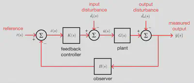
Feedback control system design
Bode, Nyquist, Nichols, root-locus plots…
Lorcan Nicholls
Graduate Engineer
An graduate engineer from the University of Cambridge. Interested in interdisciplinary engineering and science, sustainable energy and automation.